25 min read 3 hour project ~$100 Medium

Overview

If you’re training LLMs, building AI apps, or developing agents - you’ll need some way to evaluate their performance. This can come at different points in the development lifecycle: during initial development, as it’s in production to detect regressions or drift, or as you seek to upgrade to newer models and/or configurations. Because the outputs of LLMs, AI apps, and agents are typically subjective or open-ended, there are essentially only three ways performance can be measured:
  1. Human labeling or user feedback
  2. LLM-as-a-judge
  3. Vibes
Human labeling and feedback is often the most helpful, but is also the most time-consuming and expensive. Much has been written about vibes-based evals - a debate we don’t intend to get into here. This leaves us with option 2: LLM-as-a-judge, a surprisingly practical, effective, and rigorous method when done correctly. In this guide, we’ll show you a few techniques for using LLM-as-a-judge to iteratively improve your models, apps, and agents without the need for human feedback. We’ll implement them using the Sutro SDK which will make experiments fast, cheap, scalable, collaborative, easy to run - and dare we say fun?!

The Goal

We’re really going to nerd out on this one: our task today is to determine which open-source model family is best at creating ELI5 explanations of paper abstracts from the pre-print server Arxiv. ELI5 stands for “Explain Like I’m 5”, popularized by the now-defunct dataset ELI5 from Facebook. This task may seem trivial, but it’s a great demonstration of LLM-as-a-judge for a few reasons:
  1. It requires high-level world-knowledge and understanding of complex technical concepts
  2. It requires the ability to map a high-level concept to a low-level explanation and communicate it effectively
  3. It’s extremely subjective, so there is no realistic way a ground-truth label set can be created
But don’t let the specificity of the task mislead you - the following techniques can be applied to almost any scenario where you’re evaluating model, AI app, or agent performance.

Getting the data

We’ll grab the current snapshot of the Arxiv metadata from Kaggle and sample 100,000 rows.
import sutro as so
import polars as pl
import json

rows = []
with open('arxiv-metadata-oai-snapshot.json', 'r') as f:
    for line in f:
        data = json.loads(line)
        id, categories, abstract = data['id'], data['categories'], data['abstract']
        if categories and abstract:
            rows.append({'id': id, 'categories': categories, 'abstract': abstract})

df = pl.DataFrame(rows)
df.write_parquet('arxiv-metadata-id-categories-abstract-100000.snappy.parquet', compression='snappy')
Let’s briefly inspect the data to get a sense of what we’re working with.
import matplotlib.pyplot as plt
import seaborn as sns

# read the parquet file
df = pl.read_parquet('arxiv-metadata-id-categories-abstract-100000.snappy.parquet')
# cast categories to list by separating on space
df = df.with_columns(pl.col('categories').str.split(' ').alias('categories_list'))
# create high-level categories list by splitting on '.' for each item in categories_list
def get_high_level_categories(categories_list):
    return list(set([item.split('.')[0] for item in categories_list]))
df = df.with_columns(pl.col('categories_list').map_elements(get_high_level_categories).alias('high_level_categories_list'))
# explode the high_level_categories_list
df = df.explode('high_level_categories_list')
# aggregate by high_level_categories_list and count the number of papers
df = df.group_by('high_level_categories_list').agg(pl.count()).sort('count', descending=True)

# create a better looking bar chart of the high_level_categories_list
plt.figure(figsize=(12, 8))
sns.set_theme(style="whitegrid")

# Convert to pandas for seaborn
df_pandas = df.to_pandas()

# Create a more attractive bar plot
ax = sns.barplot(
    data=df_pandas, 
    x='high_level_categories_list', 
    y='count',
    palette='viridis',
    order=df_pandas.sort_values('count', ascending=False)['high_level_categories_list']
)

# Improve the styling
plt.xticks(rotation=45, ha='right')
plt.title('ArXiv High-Level Categories Distribution', fontsize=16, fontweight='bold', pad=20)
plt.xlabel('High-Level Categories', fontsize=12, fontweight='bold')
plt.ylabel('Number of Papers', fontsize=12, fontweight='bold')
# Improve layout
plt.tight_layout()

# Save with higher DPI for better quality
plt.savefig('high_level_categories_distribution.png', dpi=300, bbox_inches='tight')
Sutro Web UI
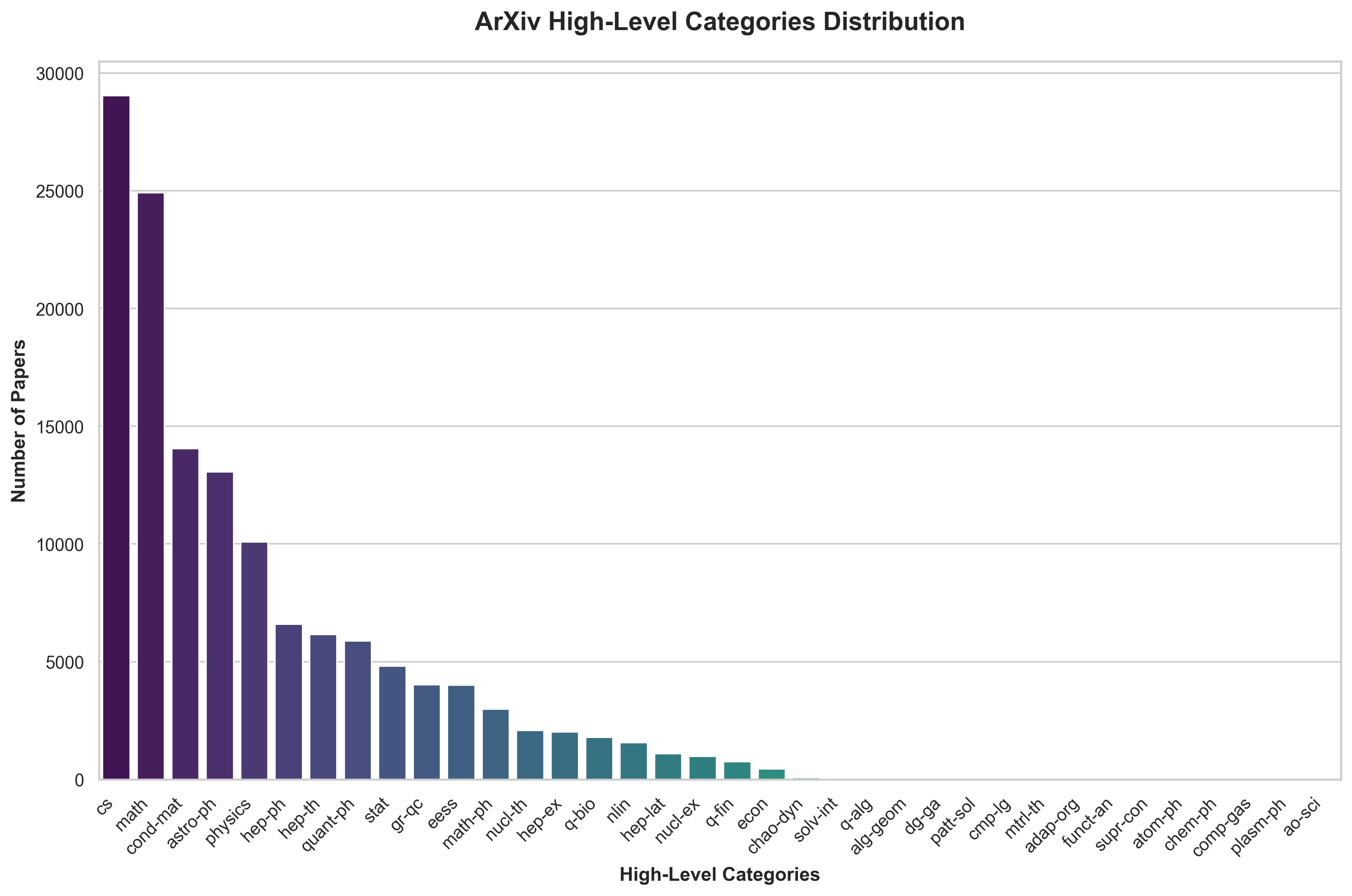
As you can see most of the high-level categories are computer science, math, and physics - with a long-tail of other more esoteric categories.

Generating the explanations

As of this writing, we serve 4 model “families” on the Sutro platform: Llama, Qwen, Gemma, and GPT-OSS. Generally speaking, any of the models should be able to generate the explanations, but the larger models should be more adept at evaluating them (larger models generally contain more world knowledge and are better at understanding complex technical concepts). So, we’ll use smaller or medium-sized variants of each model family for the explanations, and their larger counterparts for the evaluations. It’s incredibly simple to generate the explanations using the Sutro SDK. For a sanity check, we’ll run the first 1000 rows through each model using protoptying (p0) jobs.
import sutro as so

df = pl.read_parquet('arxiv-metadata-id-categories-abstract-100000.snappy.parquet')

system_prompt = """
Explain the abstract to me like I'm a 5 year old. 
Return the explanation, and nothing else.
"""

results = so.infer(
    df[0:1000],
    column='abstract',
    model=["llama-3.1-8b", "qwen-3-14b", "gemma-3-12b-it", "gpt-oss-20b"],
    system_prompt=system_prompt,
)
This kicks of four jobs in parallel each of which take just a few minutes to complete. We can inspect the results quickly and easily in the Sutro Web UI:
Sutro Web UI
An example result from GPT-OSS 20B looks like this: Input Arxiv Abstract: We report an experimental design where the position and resonance frequency of the Nitrogen Vacancy (NV) in a diamond are correlated with the room temperature. A simple model trained on the interpolated correlation data predicts both quantities. The predictive tracking of the NV's location enables continuous operation of the NV quantum computer under ambient conditions for a week without recalibration. Output ELI5 Explanation: We did a test to see how a tiny thing in a diamond moves and makes a special sound when the room is warm. We made a smart guess that tells us where it is and how it sounds. This lets a tiny computer in the diamond keep working all week without having to fix it. Scaling to the 100,000 row sample is as simple as removing the slicing of the dataframe, and setting the job priority to 1.
... previous code ...

results = so.infer(
    df,
    column='abstract',
    model=["llama-3.1-8b", "qwen-3-14b", "gemma-3-12b-it", "gpt-oss-20b"],
    system_prompt=system_prompt,
    job_priority=1,
)
This will kick off four jobs in parallel, each of which should take less than an hour to complete. In our case, here were the run stats:
ModelDurationOutput TokensCost
Llama 3.1 8B35 minutes16.3M$1.03
Qwen 3 14B48 minutes11.9M$5.76
Gemma 3 12B IT35 minutes18.8M$9.16
GPT-OSS 20B30 minutes25.8M$1.03
Let’s pull them down the explanations and append them to our original dataframe.
jobs = {
    "llama-3.1-8b": "job-c5227a15-3928-479e-a988-bef4231a9f5b",
    "qwen-3-14b": "job-a921b731-5c24-46e5-9433-c363a25777b6",
    "gemma-3-12b-it": "job-c6925843-97c8-45f8-a10a-48b17be6fa86",
    "gpt-oss-20b": "job-2b9b70f4-fd27-40d4-9f79-276b5b34df9e",
}

for model, job_id in jobs.items():
    results = so.get_job_results(job_id)
    if model == 'gpt-oss-20b': # automatically unpacks final response to content field b/c it's a reasoning model, so we handle this one differently
        results = results.with_columns(pl.col('content').alias(model))
        results = results.drop(['content', 'reasoning_content'])
    else:
        results = results.with_columns(pl.col('inference_result').alias(model))
        results = results.drop(['inference_result'])
    df = pl.concat([df, results], how='horizontal')

df.write_parquet('arxiv-metadata-id-categories-abstract-100000-explanations.parquet')

Evaluating the explanations

As mentioned earlier, it’s likely that larger models will be better at evaluating the explanations. This is because they contain more world knowledge and have more free parameters with which to reason. In some cases, you may have a “trusted” model that you want to use for all evaluations. But in this, case how do we know which model is the best judge? And how do we know the larger model in a specific family won’t be biased towards its smaller sibling due to similarities in the underlying training data? To combat these biases, we’ll use a larger model from each of the four families to evaluate the explanations from the three smaller models. Consequentially, this means that each smaller model will be evaluated by three larger models from other families. In traditional ML, this is known as ensemble modeling - using the responses of multiple models to make a single prediction.
from pydantic import BaseModel

df = pl.read_parquet('arxiv-metadata-id-categories-abstract-100000-explanations.parquet')

eval_pairs = {
    "llama-3.1-8b": ["qwen-3-32b", "gemma-3-27b-it", "gpt-oss-120b"],
    "qwen-3-14b": ["llama-3.3-70b", "gemma-3-27b-it", "gpt-oss-120b"],
    "gemma-3-12b-it": ["llama-3.3-70b", "qwen-3-32b", "gpt-oss-120b"],
    "gpt-oss-20b": ["llama-3.3-70b", "qwen-3-32b", "gemma-3-27b-it"],
}

system_prompt = """
You are a judge. You will be shown an arXiv paper abstract and an explanation of the abstract intended for a 5 year old. 
Your job is to evaluate the explanation. You should evaluate according to the following criteria:

- technical accuracy
- conceptual accuracy
- clarity
- effectiveness of communication
- overall quality

Return a score between 0 and 100, and nothing else.
"""

class Evaluation(BaseModel):
    score: int

for model, eval_models in eval_pairs.items():
    so.infer(
        df,
        column=["Abstract: ", "abstract", " Explanation: ", model],
        model=eval_models,
        system_prompt=system_prompt,
        output_schema=Evaluation,
        name=[eval_model + '_evals_' + model for eval_model in eval_models], # name the jobs so we can easily identify them
        job_priority=1,
    )
This is a very tight way to kick off the evaluation pairs! One thing you’ll notice is that we’re creating names for the jobs so we can easily identify them later. As our experimental setup grows, accurately attaching relevant metadata to each job becomes increasingly important for historical analysis, tracking, and collaboration. Sutro makes this easy. We can use the same eval mapping to pull down the results and append them to our original dataframe.
... previous code ...

jobs = so.list_jobs()
for model, eval_models in eval_pairs.items():
    for eval_model in eval_models:
        job_name = eval_model + '_evals_' + model
        job = next((job for job in jobs if job['name'] == job_name), None)
        if job:
            job_id = job['job_id']
            results = so.get_job_results(job_id)
            if eval_model == 'gpt-oss-120b': # automatically unpacks final response to content field b/c it's a reasoning model, so we handle this one differently
                results = results.with_columns(pl.col('content').alias('score'))
                results = results.with_columns(pl.col('score').struct.field('score').alias(job_name))
                results = results.drop(['content', 'reasoning_content', 'score'])
            else:
                results = results.with_columns(pl.col('score').alias(job_name))
                # drop all columns except job_name
                results = results.drop([col for col in results.columns if col != job_name])
            df = pl.concat([df, results], how='horizontal')

Each of the jobs took around an hour to complete, and cost between 4-10 dollars each. This comes out to around 50-80 dollars for all 1.2M evals spread across the 12 runs (100k rows each). We can now see how each model performed against each of its three evaluators. Let’s plot the results in a heatmap.
import pandas as pd
df = pl.read_parquet('arxiv-metadata-id-categories-abstract-100000-explanations-evals.parquet')

i_vals = sorted(list(set([eval_model for eval_models in eval_pairs.values() for eval_model in eval_models])))
j_vals = sorted(list(eval_pairs.keys()))

matrix = np.zeros((len(i_vals), len(j_vals)))
for model, eval_models in eval_pairs.items():
    for eval_model in eval_models:
        job_name = eval_model + '_evals_' + model
        scores = df[job_name]
        matrix[i_vals.index(eval_model), j_vals.index(model)] = scores.mean()

# wrap in DataFrame with labels
df_matrix = pd.DataFrame(matrix, index=i_vals, columns=j_vals)

plt.figure(figsize=(10, 8))
sns.heatmap(df_matrix, annot=True, fmt=".2f", cmap="RdYlGn", cbar=True, square=True)
plt.title("Score Matrix")
plt.xlabel("ELI5 Model")
plt.ylabel("Evaluator Model")
plt.savefig("llm-as-a-judge-score-matrix.png", dpi=300, bbox_inches='tight')
plt.show()
Heatmap of the score matrix
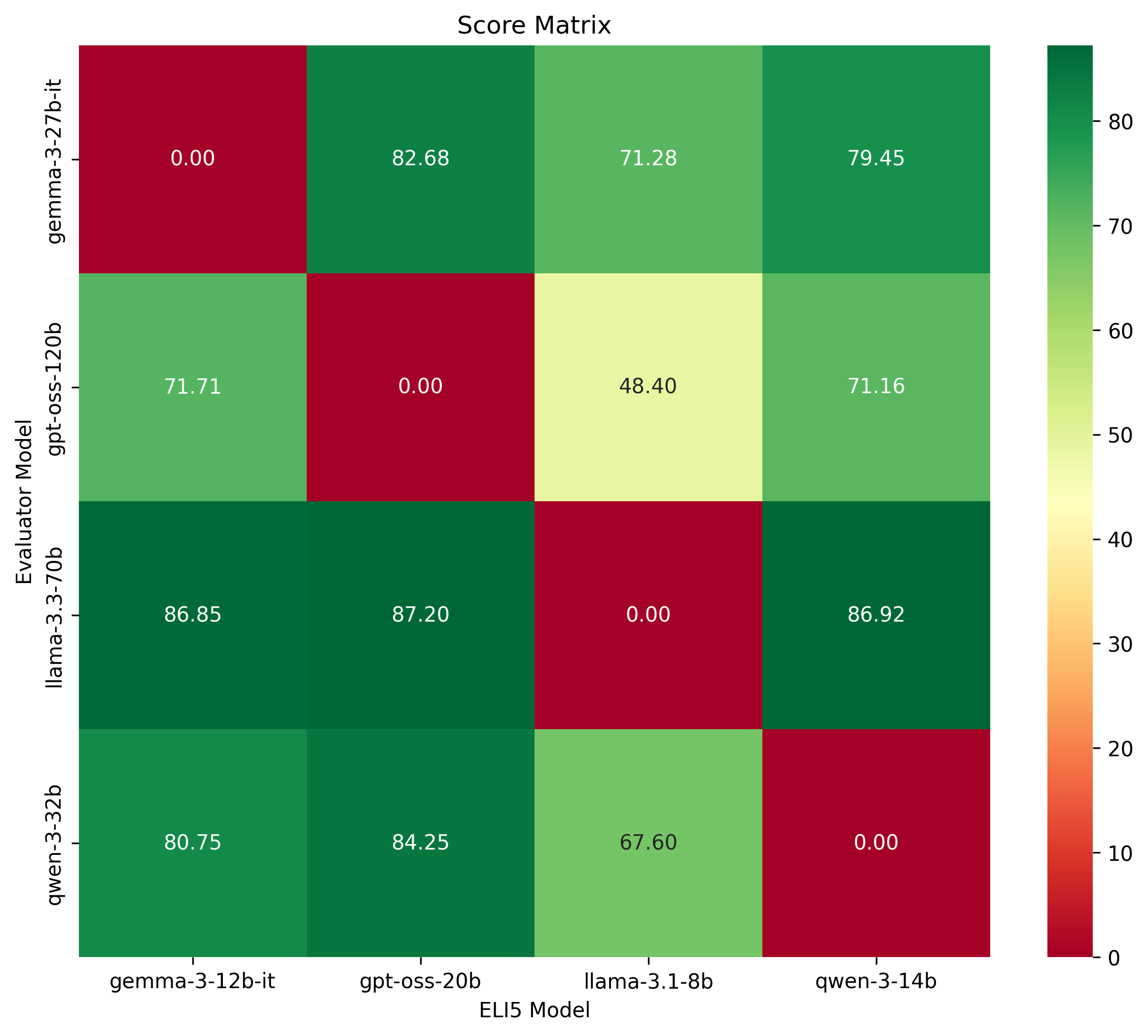
These are interesting and revealing results. We can see that the GPT-OSS 20B model has the strongest overall performance as reviewed by the three larger models in other families. The GPT-OSS 120B model is the also the harshest evaluator, giving the lowest scores to the other model families. The situation is inverted for the Llama models, where Llama 3.1 8B is the weakest performing model as reviewed by the three larger models in other families, yet Llama 3.3 70B is the most generous evaluator of the other model families. We already likely have our answer: GPT-OSS 20B is the best model for this task of the models we evaluated. At this point, we could move onto another set of evals to optimize our prompt, sampling parameters, or structured output schema. Instead, we’ll run one more set of evals to confirm our hypothesis.

Using relative evaluations

In our previous evals, we used larger models to evaluate the ELI5 explanations in isolation: just showing the abstract and the explanation to the evaluator model and asking it to score the explanation on a scale of 0 to 100. But since we’re trying to understand which model is best for our task, it makes more sense to compare relative performance directly. This is where relative evaluations come in. We’ll now show the evaluator all three ELI5 explanations at once, and ask it to rank them from best to worst.
df = pl.read_parquet('arxiv-metadata-id-categories-abstract-100000-explanations-evals.parquet')

inverse_eval_pairs = {
    "qwen-3-32b": ["llama-3.1-8b", "gemma-3-12b-it", "gpt-oss-20b"],
    "gemma-3-27b-it": ["llama-3.1-8b", "qwen-3-14b", "gpt-oss-20b"],
    "gpt-oss-120b": ["llama-3.1-8b", "qwen-3-14b", "gemma-3-27b-it"],
    "llama-3.3-70b": ["qwen-3-14b", "gemma-3-12b-it", "gpt-oss-20b"],
}

system_prompt = """
You are a judge. You will be shown an arXiv paper abstract and three explanations of the abstract intended for a 5 year old. They will be labeled as A, B, and C.

Your job is to rank the explanations from best to worst. You should evaluate according to the following criteria:

- technical accuracy
- conceptual accuracy
- clarity
- effectiveness of communication
- overall quality

You should return the ranking as a list of the labels A, B, and C, and nothing else. 

The first item in the list should be the label of the best explanation, the second item in the list should be the label of the second best explanation, and the third item in the list should be the label of the worst explanation.
"""

class Ranking(BaseModel):
    ranking: list[str]

for eval_model, eli5_models in inverse_eval_pairs.items():
    so.infer(
        df,
        column=["Abstract: ", "abstract", " Explanation A: ", eli5_models[0], " Explanation B: ", eli5_models[1], " Explanation C: ", eli5_models[2]],
        model=eval_model,
        system_prompt=system_prompt,
        output_schema=Ranking,
        name=[eval_model + '_relative_evals'],
        job_priority=1,
    )
These jobs were a bit more token heavy, but there were only four of them. However, in total all four only jobs cost around $35. We can pull down the results and append them to our original dataframe.
df = pl.read_parquet('arxiv-metadata-id-categories-abstract-100000-explanations-evals.parquet')

relative_eval_jobs = {
    "qwen-3-32b": 'job-8f460128-6426-4078-b355-7790a00c2dfa',
    "gemma-3-27b-it": 'job-5a1eed4a-44b2-4d74-a6cd-d2424e0df113',
    "gpt-oss-120b": 'job-64b2a381-5f25-4917-b2c9-78140da3c475',
    "llama-3.3-70b": 'job-2860b900-31e5-4160-b8f1-4162767215c0',
}

jobs = so.list_jobs()
for eval_model, job_id in relative_eval_jobs.items():
    eval_job_name = eval_model + '_relative_evals'
    results = so.get_job_results(job_id)
    if eval_job_name == 'gpt-oss-120b_relative_evals': # automatically unpacks final response to content field b/c it's a reasoning model, so we handle this one differently
        results = results.with_columns(pl.col('content').struct.field('ranking').alias(eval_job_name))
        results = results.drop(['content', 'reasoning_content'])
    elif eval_job_name == 'llama-3.3-70b_relative_evals': # 2 of the results had problematic json formatting, so we handle this one differently
        results = results.with_columns(
            pl.when(pl.col("inference_result").str.contains('"C", "B", "A'))
            .then(pl.lit('{"ranking": ["C", "B", "A"]}'))
            .otherwise(pl.col("inference_result"))
            .alias("inference_result")
        )
        results = results.with_columns(pl.col('inference_result').str.json_decode().alias('inference_result'))
        results = results.with_columns(pl.col('inference_result').struct.field('ranking').alias(eval_job_name))
        results = results.drop(['inference_result'])
    else:
        results = results.drop([col for col in results.columns if col != 'ranking'])
        results = results.with_columns(pl.col('ranking').alias(eval_job_name))
        results = results.drop(['ranking'])
    eli5_map = {"A": inverse_eval_pairs[eval_model][0], "B": inverse_eval_pairs[eval_model][1], "C": inverse_eval_pairs[eval_model][2]}
    results = results.with_columns(pl.col(eval_job_name).map_elements(lambda x: [eli5_map[y] for y in x]).alias(eval_job_name))
    df = pl.concat([df, results], how='horizontal')

df.write_parquet('arxiv-metadata-id-categories-abstract-100000-explanations-relative-evals.parquet')
A little more data wrangling, and we can determine the win rate percentage matrix.
df = pl.read_parquet('arxiv-metadata-id-categories-abstract-100000-explanations-relative-evals.parquet')

eval_models = inverse_eval_pairs.keys()
eli5_models = list(set([model for eval_models in inverse_eval_pairs.values() for model in eval_models]))
eli5_model_matrix = {}
for i in eli5_models:
    for j in eli5_models:
        if i != j:
            eli5_model_matrix[(i, j)] = 0

for eval_model in eval_models:
    eval_job_name = eval_model + '_relative_evals'
    eval_results = df[eval_job_name].to_list()
    for eval_result in eval_results:
        if eval_result is not None:
            eli5_model_matrix[(eval_result[0], eval_result[1])] += 1
            eli5_model_matrix[(eval_result[1], eval_result[2])] += 1
            eli5_model_matrix[(eval_result[0], eval_result[2])] += 1

win_rate_pct_matrix = {}
for i in eli5_models:
    for j in eli5_models:
        if i != j:
            num = eli5_model_matrix[(i, j)]
            den = num + eli5_model_matrix[(j, i)]
            win_rate_pct_matrix[(i, j)] = num / den if den else float('nan')

df = pd.DataFrame(np.nan, index=eli5_models, columns=eli5_models, dtype=float)
for (i, j), v in win_rate_pct_matrix.items():
    df.loc[i, j] = v
np.fill_diagonal(df.values, np.nan)  # optional: blank diagonal

plt.figure(figsize=(10, 8))
sns.heatmap(df, annot=True, fmt=".2f", cmap="RdYlGn", cbar=True, square=True)
plt.title("Win Rate Percentage Matrix (cell = P(row beats column))")
plt.xlabel("ELI5 Model (column)")
plt.ylabel("ELI5 Model (row)")
plt.savefig("llm-as-a-judge-win-rate-percentage-matrix.png", dpi=300, bbox_inches='tight')
plt.tight_layout()
plt.show()
Win rate percentage matrix
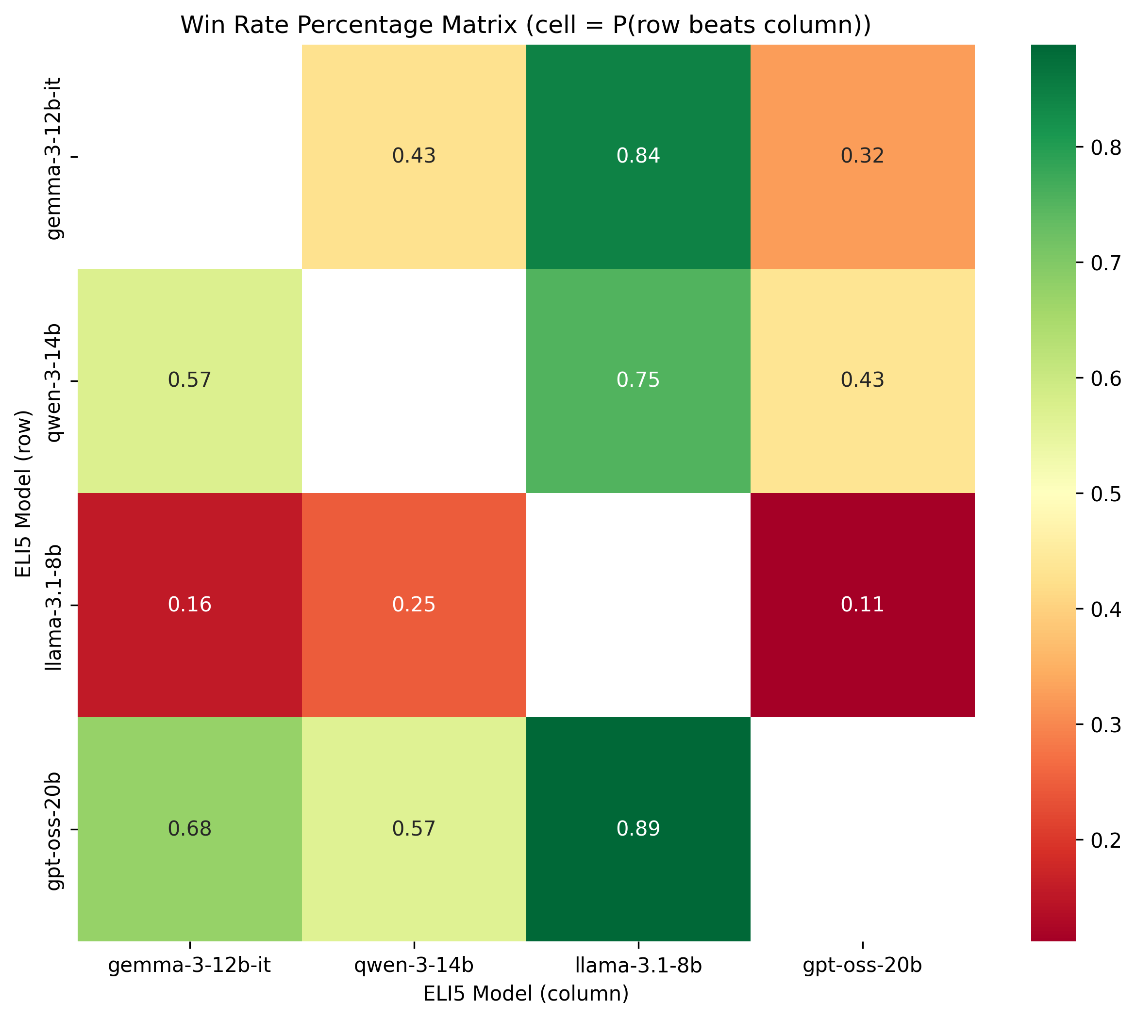
This time, we’re pooling the results of the three evaluators to determine the win rate percentage matrix. We only care about the head-to-head comparisons of the ELI5 models. Once again, even with the context of the three evaluators, we can see that GPT-OSS 20B is hands down the best model, beating all the others in head-to-head comparisons. Llama is by far the worst, getting beaten down by the others, often by a wide margin. Almost 9/10 times the GPT-OSS 20B model beats it. We like to think we’re fancy mathematicians here at Sutro, so we’ll finally use the Elo rating system to determine the best model. This is often used for human skill ratings in games like chess, and more recently to rank responses from LLMs on websites like the LM Arena Leaderboard.
import math
import numpy as np
import pandas as pd

def bt_elo_from_pair_counts(
    pair_counts: dict[tuple[str, str], int],
    ties: dict[tuple[str, str], int] | None = None,
    laplace: float = 0.5,
    max_iter: int = 1000,
    tol: float = 1e-8,
    elo_mean: float = 1500.0,
):
    """
    pair_counts: { (winner, loser): wins } for all observed directed pairs.
    ties: optional { (a, b): tie_count } counted once per unordered pair (a,b).
          If provided, each tie contributes 0.5 win to both directions.
    laplace: additive smoothing to each *directed* count (prevents zeros).
    """

    # ---- Build model list ----
    models = sorted(set([k[0] for k in pair_counts] + [k[1] for k in pair_counts]))
    m = len(models)
    idx = {name: i for i, name in enumerate(models)}

    # ---- Build directed wins matrix W[i,j] = times i beat j ----
    W = np.zeros((m, m), dtype=float)
    for (w, l), c in pair_counts.items():
        if w == l: 
            continue
        W[idx[w], idx[l]] += float(c)

    # ---- Optional ties: add 0.5 to both directions for each tie ----
    if ties:
        for (a, b), t in ties.items():
            if a == b: 
                continue
            i, j = idx[a], idx[b]
            W[i, j] += 0.5 * t
            W[j, i] += 0.5 * t

    # ---- Laplace smoothing on directed edges (excluding diagonal) ----
    if laplace and laplace > 0:
        W += laplace
        np.fill_diagonal(W, 0.0)

    # Unordered totals N_ij = W_ij + W_ji
    N = W + W.T
    np.fill_diagonal(N, 0.0)

    # Guard: drop models with zero matches
    active = (N.sum(axis=1) > 0)
    if not np.all(active):
        keep = np.where(active)[0]
        models = [models[i] for i in keep]
        idx = {name: i for i, name in enumerate(models)}
        W = W[np.ix_(keep, keep)]
        N = N[np.ix_(keep, keep)]
        m = len(models)

    # ---- Bradley–Terry via MM updates (Hunter 2004) ----
    s = np.ones(m, dtype=float)  # abilities (positive)
    for _ in range(max_iter):
        s_old = s.copy()
        w_i = W.sum(axis=1)  # total (smoothed) wins per model
        # denom_i = sum_j N_ij / (s_i + s_j)
        denom = (N / (s.reshape(-1,1) + s.reshape(1,-1) + 1e-12)).sum(axis=1)
        upd = denom > 0
        s[upd] = w_i[upd] / denom[upd]
        # normalize to keep scale stable (geometric mean = 1)
        s /= np.prod(s) ** (1.0 / m)
        if np.max(np.abs(np.log(s + 1e-12) - np.log(s_old + 1e-12))) < tol:
            break

    # ---- Convert to beta and Elo-like ratings ----
    beta = np.log(s + 1e-12)
    elo = (400.0 / math.log(10.0)) * beta
    elo = elo - np.mean(elo) + elo_mean  # center

    # ---- Summaries and expected probabilities ----
    wins = W.sum(axis=1)
    losses = W.sum(axis=0)
    matches = N.sum(axis=1)  # unordered total vs all opponents

    ratings = pd.DataFrame({
        "ability": s,
        "beta": beta,
        "elo": elo,
        "wins": wins,
        "losses": losses,
        "matches": matches,
    }, index=models).sort_values("elo", ascending=False)

    P = s.reshape(-1,1) / (s.reshape(-1,1) + s.reshape(1,-1))
    np.fill_diagonal(P, np.nan)
    p_matrix = pd.DataFrame(P, index=models, columns=models)

    return ratings, p_matrix

ratings, p_exp = bt_elo_from_pair_counts(eli5_model_matrix, ties=None)
print(ratings[["elo","wins","losses","matches"]].to_markdown())
We get the following results:
elowinslossesmatches
gpt-oss-20b1629.77425974174028600001
qwen-3-14b1554.52351422248580600001
gemma-3-12b-it1523.23319396280606600003
llama-3.1-8b1292.47103212496790600001
The results are clear - GPT-OSS 20B is the clear winner, followed by Qwen 3 14B, and then Gemma 3 12B. Llama 3.1 8B is the worst performer.

Conclusion

We just demonstrated how you can use Sutro to run model task evals. Our approach avoided the need for human feedback altogether, instead using an ensemble of LLMs to evaluate our task and remove the biases of any single model. This avoided the need for human labelers, or any online human feedback. We bootstrapped the evaluation process entirely offline:
  • in just a few hours
  • on 100,000 samples, across 4 models and 16 evaluation jobs (but could be scaled to millions of samples and billions of tokens)
  • for around 100 dollars
  • without the need for any custom infrastructure or GPU setup
  • using only the Sutro SDK and open-source Python tools

Next Steps

While we identified a good base model to start with, a good next step might be to use our winning model, and run further offline evals to improve prompts, sampling parameters, or structured output schemas - taking our task specification to a truly optimized state. And to reiterate once more - this iterative, offline eval process can be used to improve nearly any AI application or agent, including but not limited to:

New model development and benchmarking:

You can continuously run large scale evals as you post-train, fine-tune, and improve your models without human feedback.

Task specialization:

When trying to optimize an LLM task such as summarization, classification, or code-generation, you can evaluate your choice of model, prompt, sampling parameters, and more to optimize selections and maximize performance.

Application and agent development/tuning:

As you create more complex, compound, and agentic tasks, you can evaluate entire reasoning traces, workflow outputs, and application logs to tune performance without the need for human feedback. Hopefully this helps get you started with LLM-as-a-judge methods on the Sutro platform. We encourage you to bring your own approaches, and get creative with the task you’re trying to evaluate. If you need any help getting started, contact us at team@sutro.sh. You can review the full, resulting MIT-licensed dataset associated with this guide here: